
Mastering Excel Filter Function: Streamline Your Data Like a Pro!
- Zainab

- Apr 8, 2023
- 4 min read
Updated: Nov 14, 2023
A data analyst tracking data in a spreadsheet may want to get a subset of the data to gain insights, especially if the dataset is large.
This is where a filter function comes to the rescue.
Filters can quickly sort and display specific data within a larger dataset.
You can select columns, rows or cells within a range of data and return only those that meet your specified criteria.
The filter condition can be easily modified, allowing you to be more flexible when analysing your data. This is useful when working with dynamic data or conducting iterative analysis.
Let's explore some different combinations of filter functions and other conditions.
Below is a fictitious sales dataset I created to illustrate this.
It shows the salespersons, the regions they operate in, the products they've sold, and the revenue and profit generated from each sale in Ghanaian Cedi.

This is a general syntax for the Filter function.
=FILTER(array, include, [if_empty])array: This is the range or array of data that you want to filter.
include: This is the criteria that the data in the array must meet to be included in the filtered result. It can be a logical expression, an array of TRUE/FALSE values, or a range of cells containing TRUE/FALSE values.
[if_empty]: (Optional) This argument specifies the value to be returned if no results meet the filtering criteria. If omitted, the function returns an error if no results are found.
In the first example, only the filter function will be used.
Question: Who are the salespersons that sold only ovens?
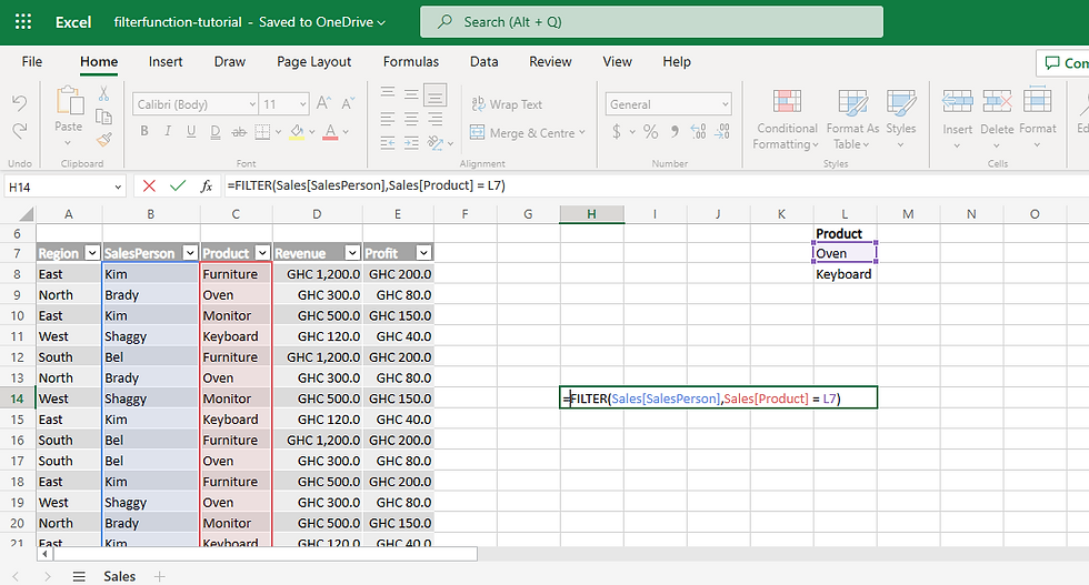
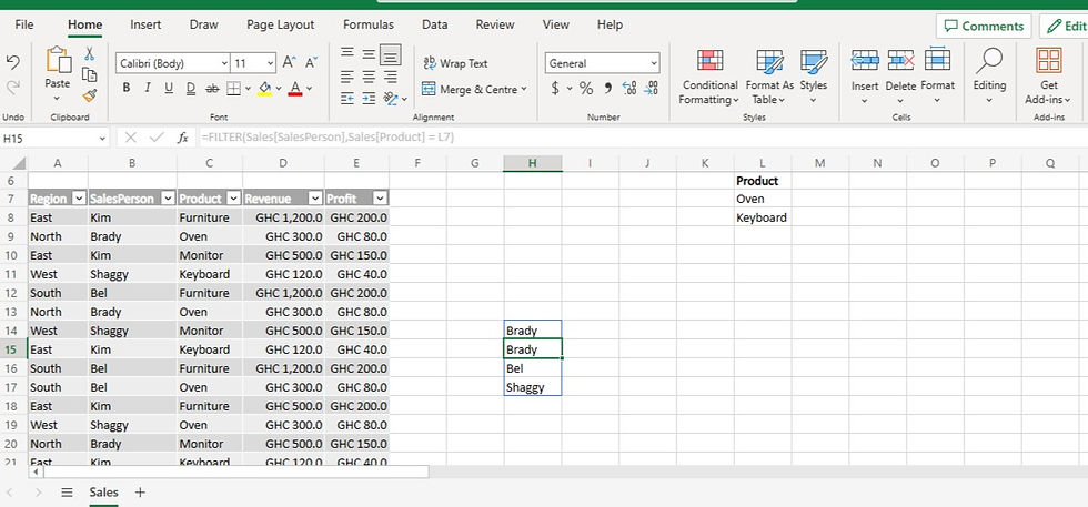
It returns all cells that meet the criteria regardless of duplicates. There has been more than one instance where "Brady" has sold an oven.
In this part of the demo, I'll use the UNIQUE and INDEX functions in conjunction with the Filter function to return values that meet the criteria.
The UNIQUE function returns a list of unique values or ranges.
The INDEX function returns a value or the reference to a value from within a table or range.
Now, let's incorporate the INDEX function.
Question: Which salesperson's name appeared first among those who sold ovens?

The formula returns the first value (Brady) regardless of the number of values in the filtered range.

If the function needed to find the first two cells in the filtered range, it would have been modified accordingly:
=INDEX(FILTER(Sales[SalesPerson],Sales[Product] = L7),{1,2})This would have returned "Brady" twice because that's the first two cells in the filtered range.
We could also return the first and third cells with a function like this:
=INDEX(FILTER(Sales[SalesPerson],Sales[Product] = L7),{1,3})The values returned would be "Brady" and "Bel".
Next, using the UNIQUE function, return all the names of salespeople who sold ovens.

Now we have unique names of salespersons who sold ovens. Although "Brady" appears twice in the dataset, only one instance was returned.

We have been returning single values. Let's define a condition that retrieves a subset of the data when the criteria are met.
To return a range of values, we need to input the table's name as the first argument to the function.
Question: Find all rows that have "East" as a region.

As a result, rows with the region as "East" were returned. In this region, "Kim" is the only salesperson.

Let's add in some logical conditions ( AND, OR operations).
Consider the "OR" condition. The + sign denotes it.
It returns True if at least one condition is met.
Question: Find all rows that have either "Monitor" or "Keyboard" as a product

Our result shows six rows.

The "AND" condition returns True when all criteria are met. Denoted by the * sign
Question: Find all rows with the region "North" AND a profit amount greater than GHC100.

Our function only returns a row. Only this row met both criteria.

The final condition we'll look at is the "NOT" condition denoted by <>. It negates a specified criterion and returns False if it is True, and vice versa.
In this case, it will be used with the AVERAGE function to return a single value.
Question: Find the average revenue where the Product is Not "Furniture".

This returns a single number because we wanted the average of all the revenue where a product is not Furniture. If the AVERAGE function is omitted, it will list all revenue amounts that meet this condition.

Let's finish up with a combination of the logical conditions.
Question: Which records have either "West" or "South" as a region but not "Furniture" as a product?

Here, we have four records that meet the condition.

How to handle errors in filter functions
The filter function allows for a third parameter. It returns that specified value when there is an error.
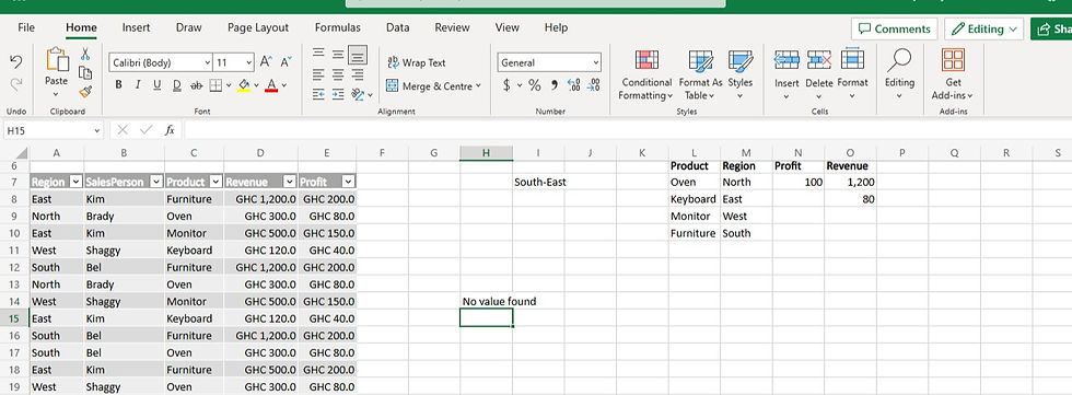
Let's put this to the test with a criterion that looks for a value that is not in the data or filtered range.
There is no "South-East" in the region column.
Question: What records have "South-East" as a region and products not "Furniture"
This is the formula without specifying a value.

It shows a CALC error. This error occurs when Excel's calculation engine encounters an unspecified calculation error with an array.

This time, include the value to return when there is an error.

Here, it returns "No value Found". This value can be replaced with any value of your choice or an empty string.
In general, functions can improve calculation accuracy by removing human error. They are programmed to perform specific tasks accurately and consistently, which reduces the likelihood of mistakes in your work.
Additionally, they can be used to validate data entries, ensuring they meet specific criteria or requirements.
Using Excel functions can help you save time, reduce errors, and make better decisions based on accurate and reliable data analysis.
Hopefully, you have gained some vital information from this read.
Until next time, keep excelling!
Comments